Exploring Indian Food Composition with thali
Source:vignettes/thali-overview.Rmd
thali-overview.Rmd
library(thali)
library(dplyr)
library(tidyr)
library(ggplot2)
library(ggrepel)
library(scales)
library(patchwork)
library(forcats)

data_available <- tryCatch(
  {
    nrow(thali_proximate) > 0
  },
  error = function(e) FALSE
)
knitr::opts_chunk$set(eval = data_available)
thali provides programmatic access to the Indian
Food Composition Tables (IFCT) 2017, published by the National
Institute of Nutrition (NIN), ICMR, Hyderabad. It covers 528 Indian
foods across 12 nutrient categories.
The package is named after the colloquial Indian thali, a meal on one plate.
1. Browsing the database
foods <- list_foods()

group_counts <- foods |>
  count(food_group, name = "n_foods") |>
  arrange(desc(n_foods))

ggplot(group_counts, aes(
  x = reorder(food_group, n_foods), y = n_foods,
  fill = food_group
)) +
  geom_col(width = 0.7, show.legend = FALSE) +
  geom_text(aes(label = n_foods), hjust = -0.2, size = 3.2, colour = "#333333") +
  scale_fill_manual(values = food_group_colours()) +
  scale_y_continuous(expand = expansion(mult = c(0, 0.12))) +
  coord_flip() +
  labs(
    title    = "IFCT 2017: Food items by group",
    x        = NULL,
    y        = "Number of foods",
    caption  = "Source: NIN/ICMR, Indian Food Composition Tables 2017"
  ) +
  theme_thali()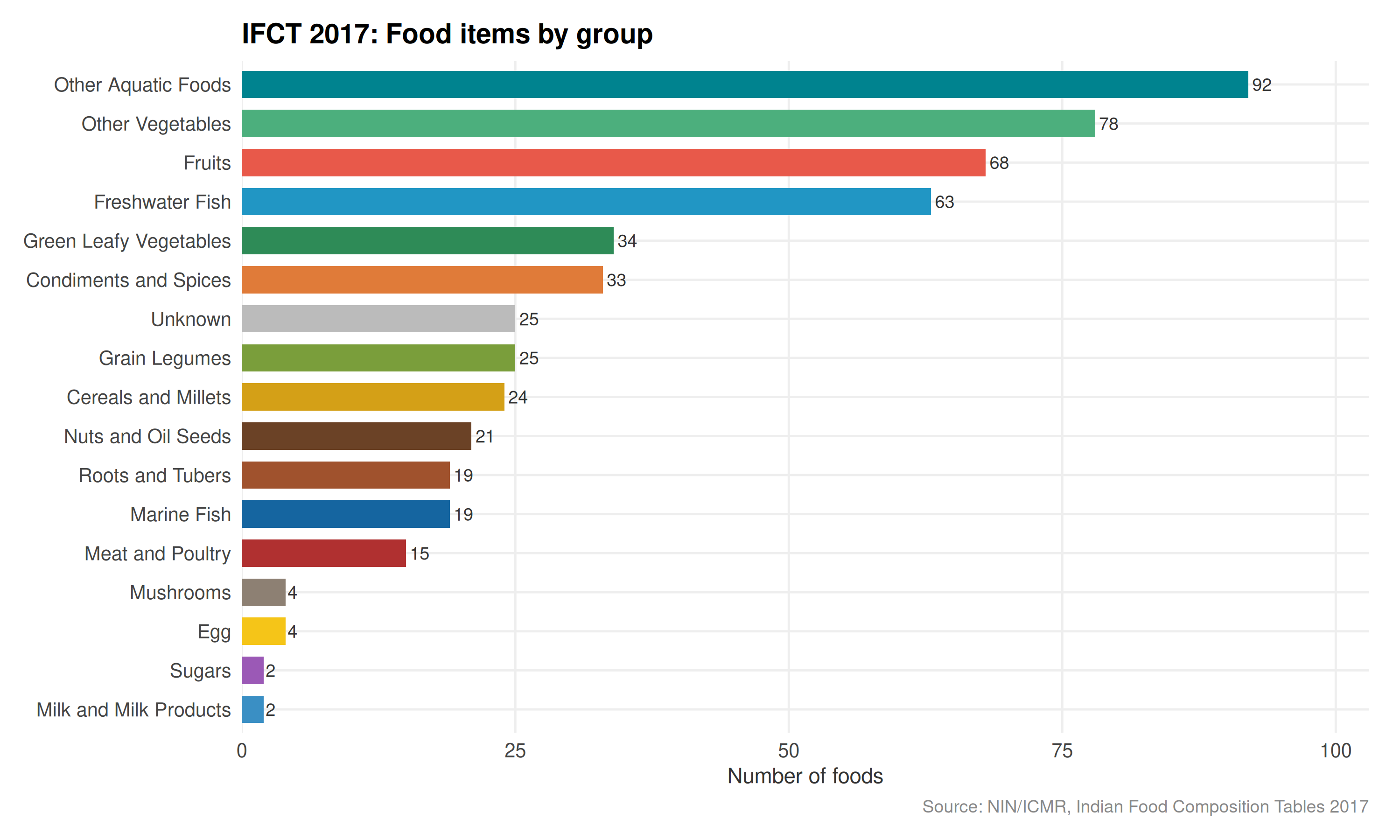
search_food("dal")
#> # A tibble: 8 × 3
#>   food_code food_name                             food_group
#>   <chr>     <chr>                                 <chr>
#> 1 B001      "Bengal gram, dal (Cicer arietinum)"  Grain Legumes
#> 2 B003      "Black gram, dal (Phaseolus mungo)"   Grain Legumes
#> 3 B010      "a)\nGreen gram, dal (\nVigna radiat" Grain Legumes
#> 4 B013      "Lentil dal (Lens culinaris)"         Grain Legumes
#> 5 B021      "Red gram, dal (Cajanus cajan)"       Grain Legumes
#> 6 H001      "Almond (Prunus amygdalus)"           Nuts and Oil Seeds
#> 7 P020      "(Synodus indicus)\nKadal bral"       Other Aquatic Foods
#> 8 P021      "Kadali (Nemipterus mesoprion)"       Other Aquatic Foods
list_nutrients("amino_acids")
#> # A tibble: 18 × 2
#> table nutrient
#> <chr> <chr>
#> 1 amino_acids Histidine_HIS(g)
#> 2 amino_acids Isoleucine_ILE(g)
#> 3 amino_acids Leucine_LEU(g)
#> 4 amino_acids Lysine_LYS(g)
#> 5 amino_acids Methionine_MET(g)
#> 6 amino_acids Cysteine_CYS(g)
#> 7 amino_acids Phenylalanine_PHE(g)
#> 8 amino_acids Threonine_THR(g)
#> 9 amino_acids Tryptophan_TRP(g)
#> 10 amino_acids Valine_VAL(g)
#> 11 amino_acids Alanine_ALA(g)
#> 12 amino_acids Arginine_ARG(g)
#> 13 amino_acids AsparticAcid_ASP(g)
#> 14 amino_acids GlutamicAcid_GLU(g)
#> 15 amino_acids Glycine_GLY(g)
#> 16 amino_acids Proline_PRO(g)
#> 17 amino_acids Serine_SER(g)
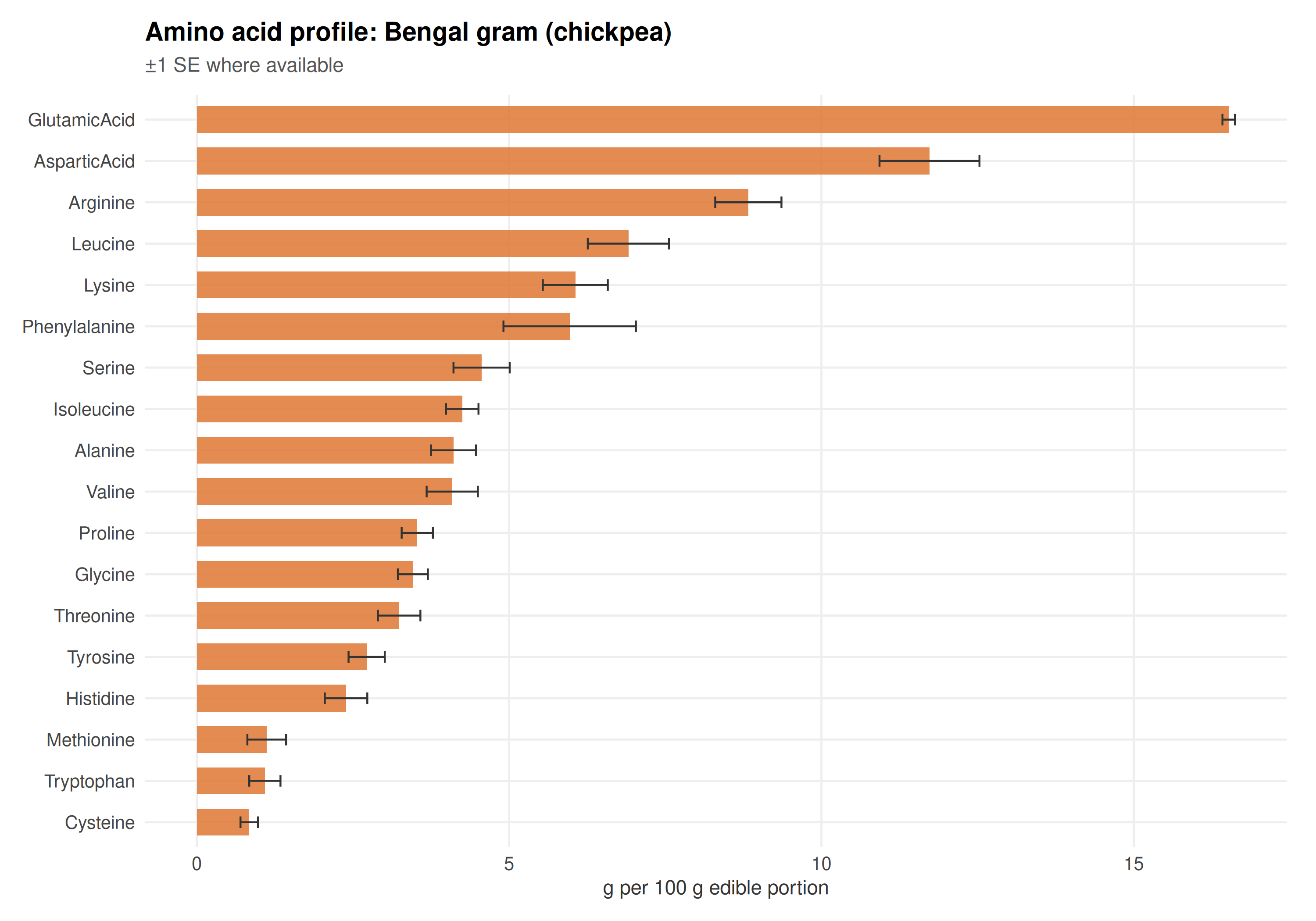
#> 18 amino_acids Tyrosine_TYR(g)2. Single-food nutrient profile: Bengal gram (chickpea)
plot_composition(
  food     = "Bengal gram",
  table    = "amino_acids",
  label_fn = function(x) gsub("_.*", "", x),
  title    = "Amino acid profile: Bengal gram (chickpea)",
  xlab     = "g per 100 g edible portion"
)
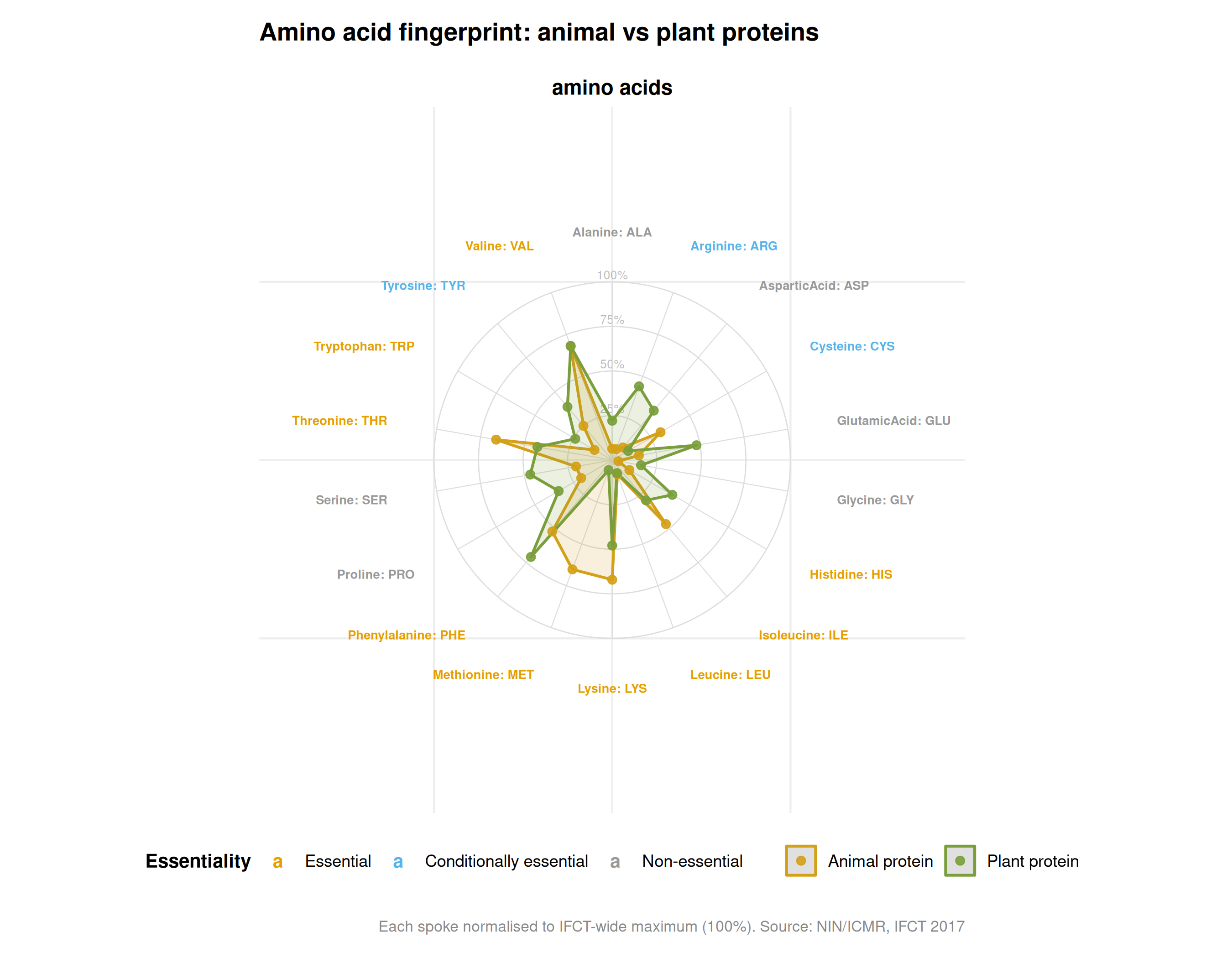
3. Animal vs plant protein: amino acid fingerprint
Animal proteins (egg, chicken, milk) supply all essential amino acids in substantial amounts. Plant proteins (legumes) are often limiting in one or two acids, particularly methionine and lysine. The radar shows the average amino acid fingerprint of each group, normalised to the IFCT-wide maximum so the shape differences are directly comparable.
avg_meal <- function(food_names) {
  portions <- setNames(rep(100, length(food_names)), food_names)
  compose_meal(portions)
}

animal_meal <- avg_meal(c(
  "Egg, poultry, whole, boiled",
  "Chicken, poultry, breast, skinless",
  "Milk, whole, Cow"
))

plant_meal <- avg_meal(c(
  "Bengal gram, whole",
  "Lentil dal",
  "Soybean, brown",
  "Red gram, dal"
))

thali_plot(
  list(`Animal protein` = animal_meal, `Plant protein` = plant_meal),
  tables = "amino_acids",
  title = "Amino acid fingerprint: animal vs plant proteins",
  base_size = 11,
  ncol = 1L
)
4. Macronutrient profiles of Indian staples
staples <- c(
  "Rice", "Wheat flour", "Jowar", "Bajra", "Ragi",
  "Bengal gram", "Red gram", "Black gram"
)

macro_data <- lapply(staples, function(food) {
  d <- get_nutrition(food, table = "proximate")
  if (nrow(d) == 0) {
    return(NULL)
  }
  d[1, ]
}) |>
  bind_rows() |>
  select(`Food name`,
    Protein = `Protein_PROTCNT(g)`,
    Fat     = `TotalFat_FATCE(g)`,
    Carbs   = `AvailableCarbohydrate_CHOAVLDF(g)`,
    Fibre   = `TotalDietaryFibre_FIBTG(g)`
  ) |>
  mutate(across(c(Protein, Fat, Carbs, Fibre), as.numeric)) |>
  pivot_longer(c(Protein, Fat, Carbs, Fibre),
    names_to = "macro", values_to = "value"
  ) |>
  filter(!is.na(value)) |>
  mutate(
    `Food name` = gsub(", whole|, raw| grain| flour", "", `Food name`),
    macro = forcats::fct_reorder(macro, value, sum)
  )

carb_order <- macro_data |>
  filter(macro == "Carbs") |>
  arrange(value) |>
  pull(`Food name`)

ggplot(
  macro_data,
  aes(x = factor(`Food name`, levels = carb_order), y = value, fill = macro)
) +
  geom_col(position = "stack", width = 0.7, alpha = 0.9) +
  scale_fill_manual(
    values = c(
      Carbs = "#D4A017", Protein = "#3A8FC4",
      Fat = "#E07B39", Fibre = "#2E8B57"
    ),
    name = NULL
  ) +
  coord_flip() +
  labs(
    title = "Macronutrient composition of Indian staple cereals and pulses",
    subtitle = "g per 100 g edible portion",
    x = NULL, y = "g per 100 g",
    caption = "Source: NIN/ICMR, IFCT 2017"
  ) +
  theme_thali() +
  theme(legend.position = "top")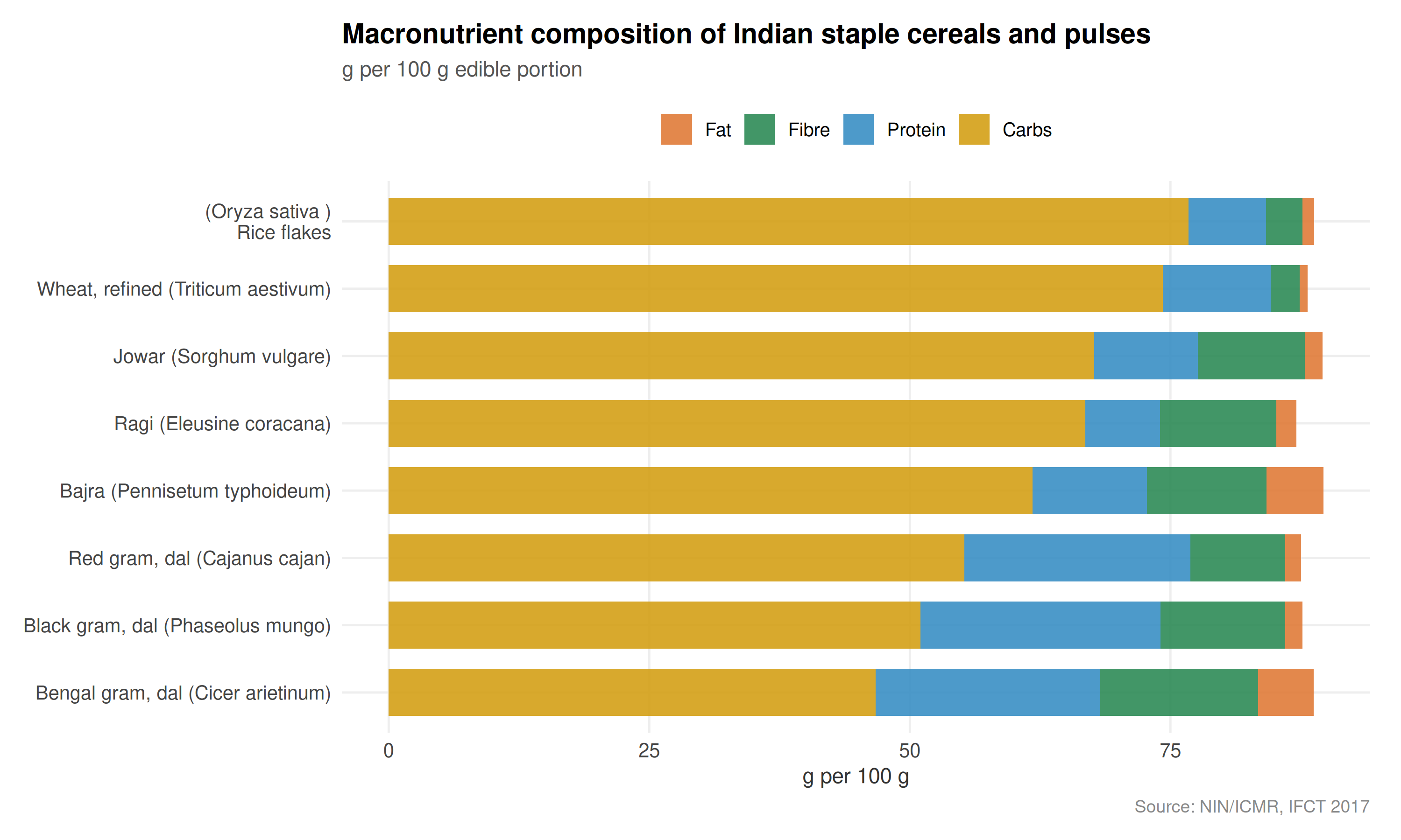
5. Top-protein foods by food group
prot <- thali_proximate |>
  mutate(
    protein    = as.numeric(`Protein_PROTCNT(g)`),
    food_group = decode_food_code(`Food code`)
  ) |>
  filter(!is.na(protein)) |>
  group_by(food_group) |>
  slice_max(protein, n = 1) |>
  ungroup() |>
  arrange(desc(protein)) |>
  filter(!food_group %in% c("Unknown", "Sugars", "Edible Oils and Fats"))

ggplot(prot, aes(x = reorder(`Food name`, protein), y = protein, fill = food_group)) +
  geom_col(width = 0.7, alpha = 0.9, show.legend = FALSE) +
  geom_label_repel(
    aes(label = food_group),
    nudge_x = 0.5, direction = "y", hjust = 0,
    size = 2.8, label.size = 0, fill = "white",
    alpha = 0.85, colour = "#333333", max.overlaps = 20
  ) +
  scale_fill_manual(values = food_group_colours()) +
  scale_y_continuous(expand = expansion(mult = c(0, 0.3))) +
  coord_flip() +
  labs(
    title = "Highest-protein food in each IFCT food group",
    subtitle = "Protein (g per 100 g edible portion)",
    x = NULL, y = "Protein (g/100 g)",
    caption = "Source: NIN/ICMR, IFCT 2017"
  ) +
  theme_thali()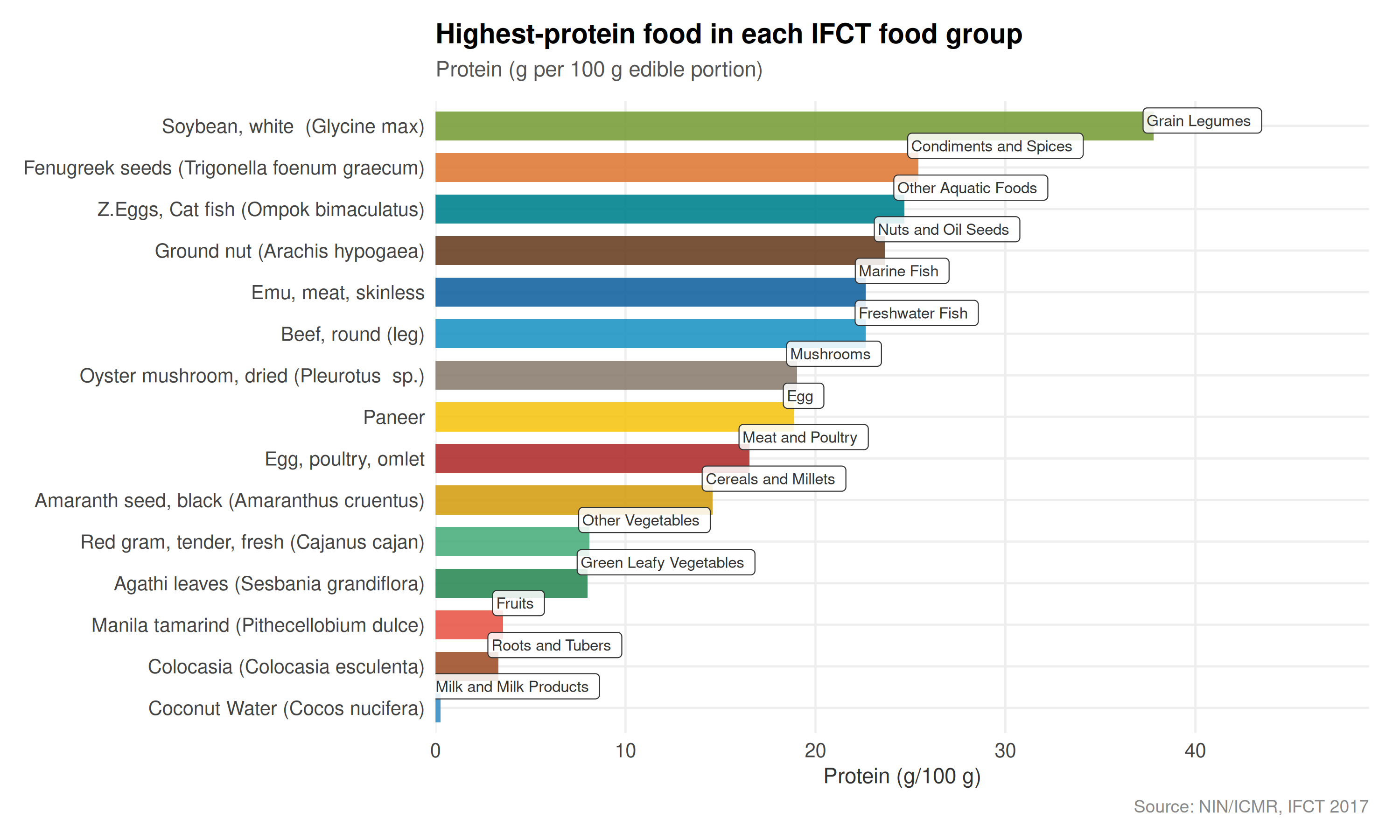
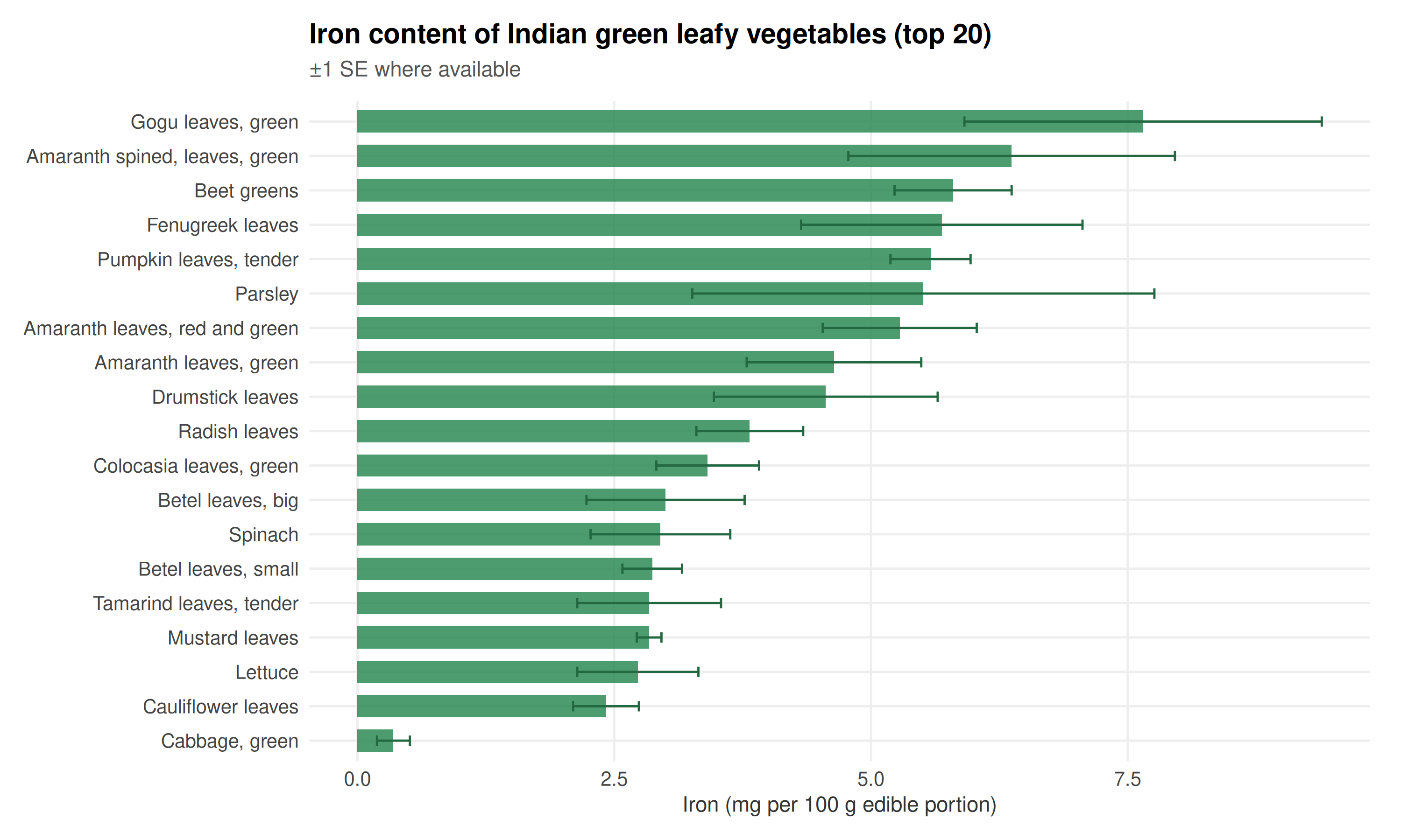
6. Iron in leafy vegetables
plot_ranked(
  table      = "minerals",
  nutrient   = "Iron_Fe(mg)",
  se_table   = thali_minerals_se,
  food_group = "Green Leafy Vegetables",
  fill       = "#2E8B57",
  title      = "Iron content of Indian green leafy vegetables (top 20)",
  xlab       = "Iron (mg per 100 g edible portion)"
)
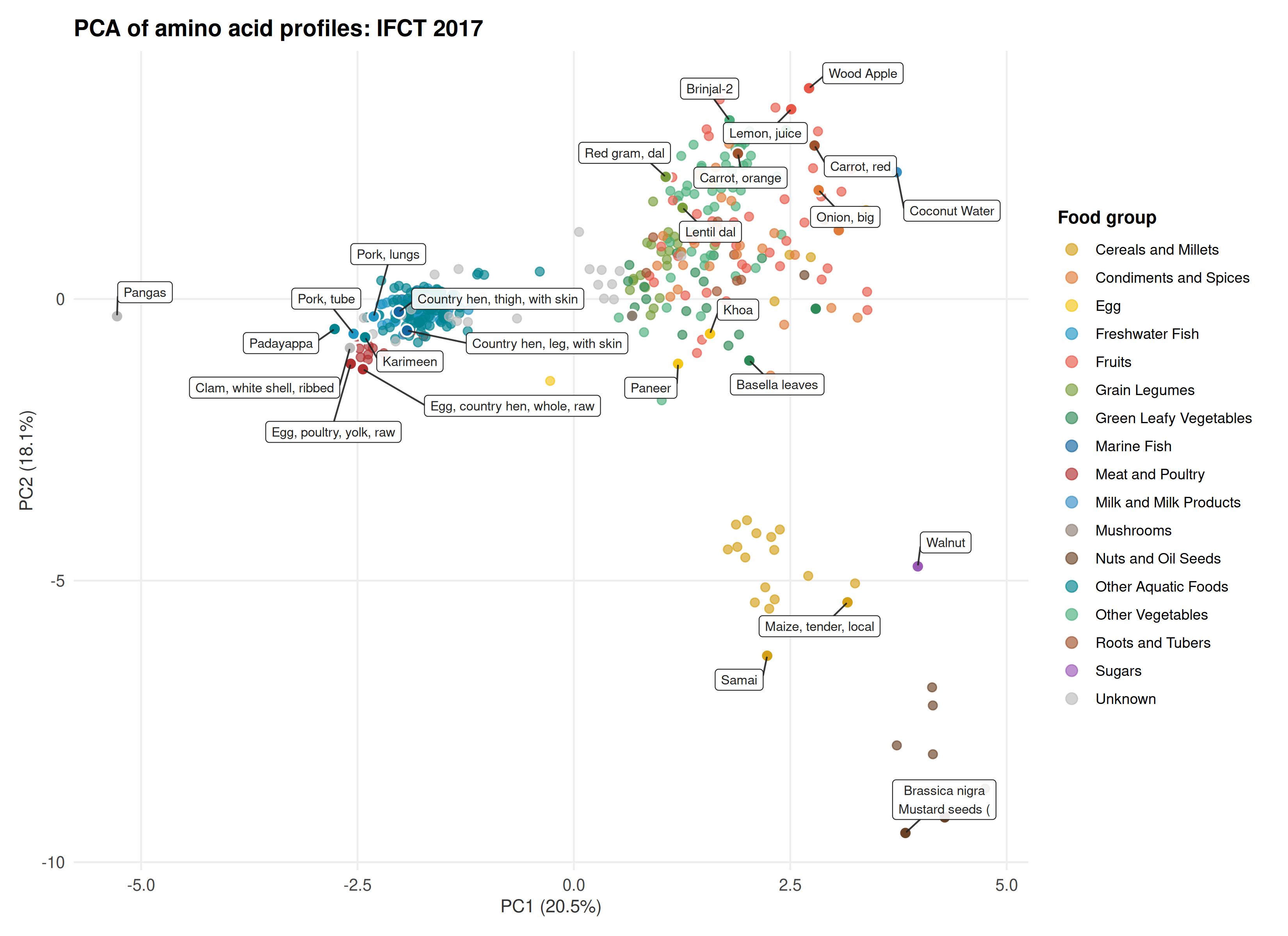
7. Amino acid profiles across food groups
pca_aa <- run_pca("amino_acids", min_obs = 8L)
plot_pca(pca_aa,
  title = "PCA of amino acid profiles: IFCT 2017"
)
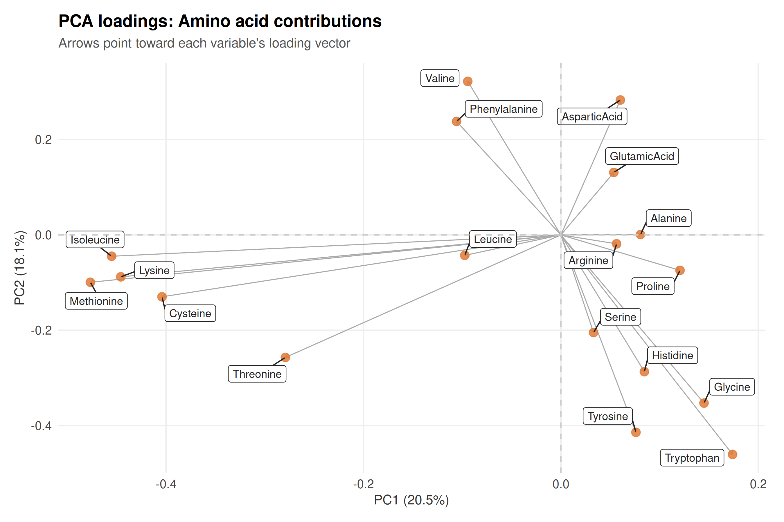
plot_pca_loadings(pca_aa,
  title = "PCA loadings: Amino acid contributions"
)
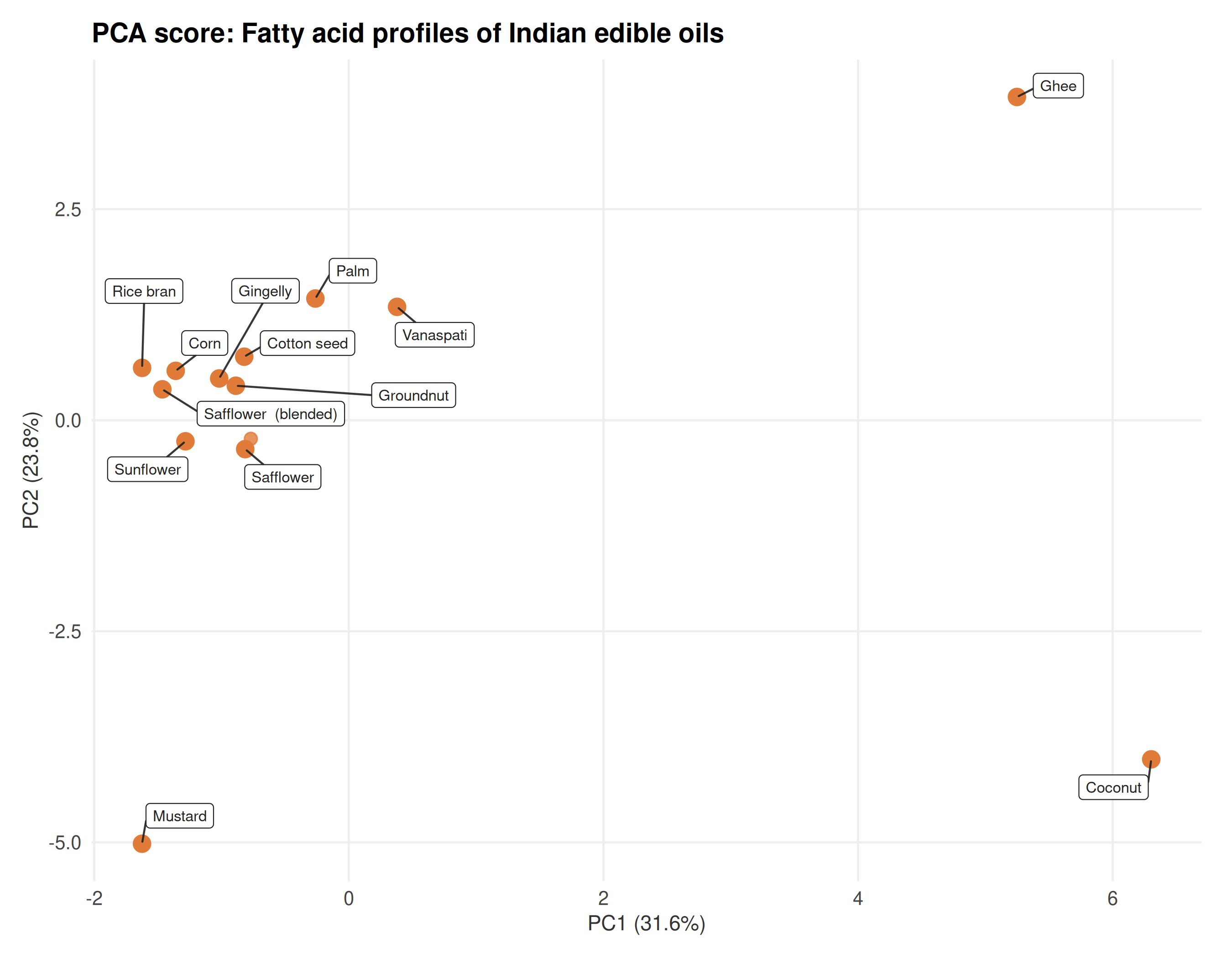
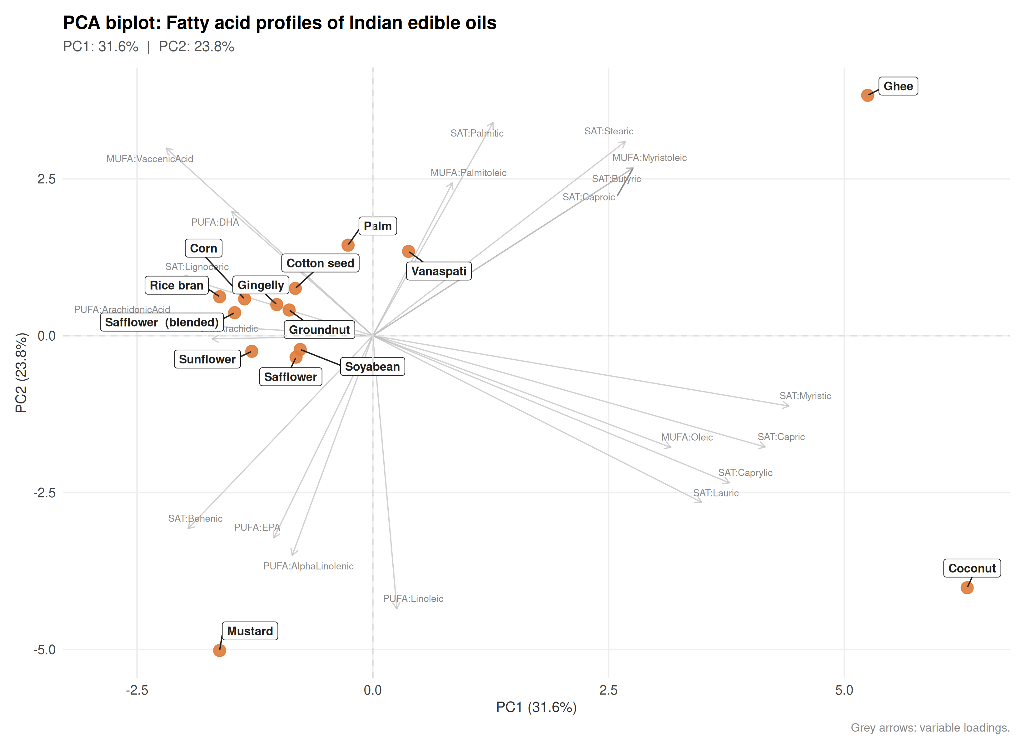
8. Fatty acid profiles of edible oils
oil_label_fn <- function(x) gsub(",.*|[Oo]il|[Ff]at", "", x) |> trimws()
fa_label_fn <- function(x) {
  x |>
    gsub("Saturated_", "SAT:", x = _) |>
    gsub("Monounsaturated_", "MUFA:", x = _) |>
    gsub("Polyunsaturated_", "PUFA:", x = _) |>
    gsub("_C.*", "", x = _)
}

pca_oils <- run_pca(
  "edible_oils",
  drop_cols = c("Total_MUFA(%)", "Total_PUFA(%)"),
  impute    = "zero",
  group_col = FALSE,
  min_obs   = 4L
)
plot_pca(pca_oils,
  label_fn = oil_label_fn,
  n_label  = 13L,
  title    = "PCA score: Fatty acid profiles of Indian edible oils"
)
plot_pca_biplot(
  pca_oils,
  score_label_fn = oil_label_fn,
  load_label_fn = fa_label_fn,
  title = "PCA biplot: Fatty acid profiles of Indian edible oils"
)
9. Saturated vs unsaturated fatty acids : edible oils
# Use Total_MUFA(%) and Total_PUFA(%) as authoritative class totals;
# Saturated = 100 - MUFA - PUFA (individual FAs are incomplete, summing them
# over-counts or under-counts depending on which are reported).
class_totals <- thali_edible_oils |>
  mutate(
    mufa = as.numeric(`Total_MUFA(%)`),
    pufa = as.numeric(`Total_PUFA(%)`),
    sat = 100 - mufa - pufa,
    oil_short = gsub(",.*|[Oo]il|[Ff]at", "", `Food name`) |> trimws()
  ) |>
  filter(!is.na(mufa), !is.na(pufa)) |>
  select(oil_short, Saturated = sat, MUFA = mufa, PUFA = pufa) |>
  pivot_longer(c(Saturated, MUFA, PUFA), names_to = "fa_class", values_to = "pct") |>
  mutate(fa_class = factor(fa_class, levels = c("PUFA", "MUFA", "Saturated")))

sat_order <- class_totals |>
  filter(fa_class == "Saturated") |>
  arrange(pct) |>
  pull(oil_short)

ggplot(
  class_totals,
  aes(x = factor(oil_short, levels = sat_order), y = pct, fill = fa_class)
) +
  geom_col(position = "stack", width = 0.7, alpha = 0.9) +
  scale_fill_manual(
    values = c(Saturated = "#B03030", MUFA = "#E07B39", PUFA = "#2E8B57"),
    name = "Fatty acid class"
  ) +
  scale_y_continuous(
    labels = label_percent(scale = 1),
    limits = c(0, 100),
    expand = expansion(mult = c(0, 0.02))
  ) +
  coord_flip() +
  labs(
    title = "Fatty acid class composition of Indian edible oils",
    subtitle = "% of total fatty acid methylesters (Saturated = 100 − MUFA − PUFA)",
    x = NULL, y = "% of total FA",
    caption = "Source: NIN/ICMR, IFCT 2017"
  ) +
  theme_thali() +
  theme(legend.position = "top")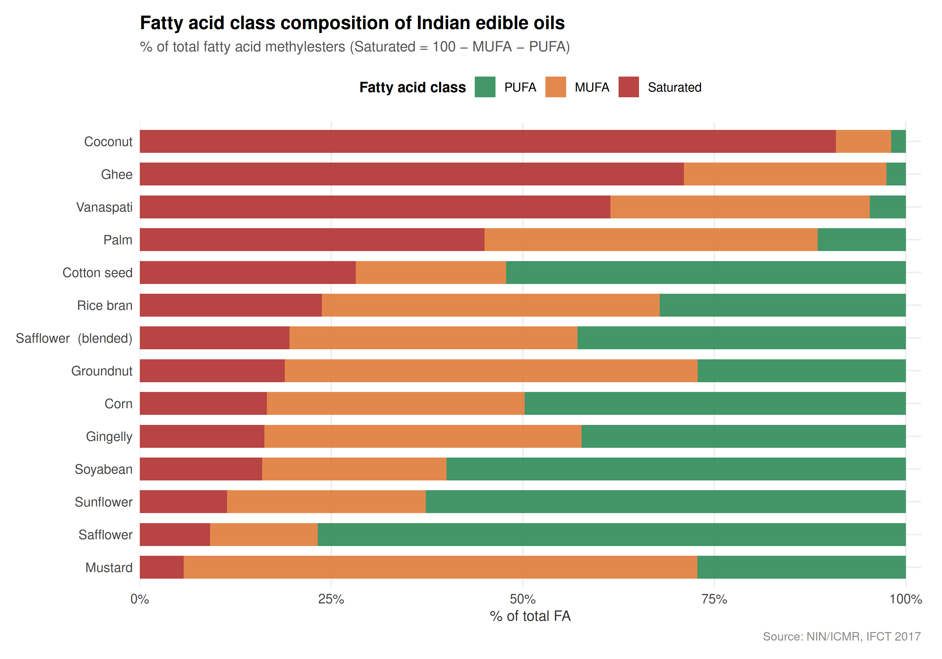
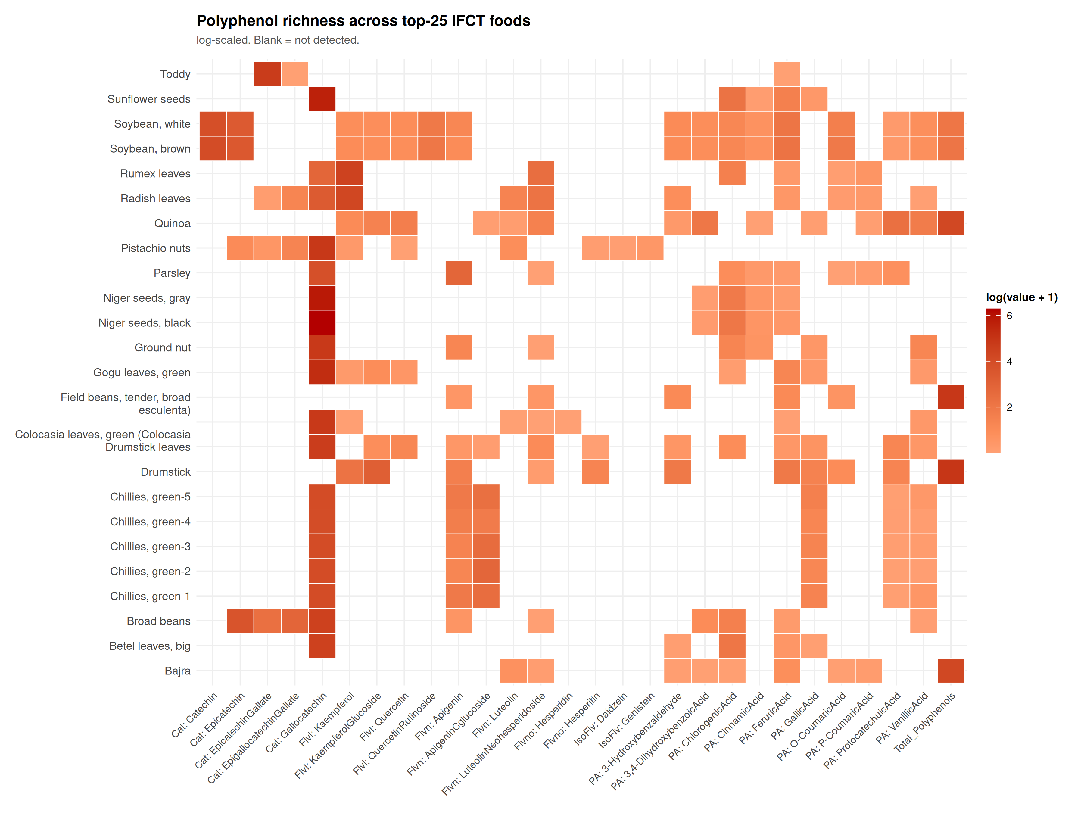
10. Polyphenol richness heatmap
plot_heatmap(
  "polyphenols",
  n = 25L,
  var_label_fn = function(x) {
    x |>
      gsub("PhenolicAcid_", "PA: ", x = _) |>
      gsub("Flavone_", "Flvn: ", x = _) |>
      gsub("Flavonol_", "Flvl: ", x = _) |>
      gsub("Flavanone_", "Flvno: ", x = _) |>
      gsub("Isoflavone_", "IsoFlv: ", x = _) |>
      gsub("Catechin_", "Cat: ", x = _) |>
      gsub("_[A-Z]+\\(mg\\)", "", x = _) |>
      gsub("\\(mg\\)", "", x = _)
  },
  title = "Polyphenol richness across top-25 IFCT foods"
)
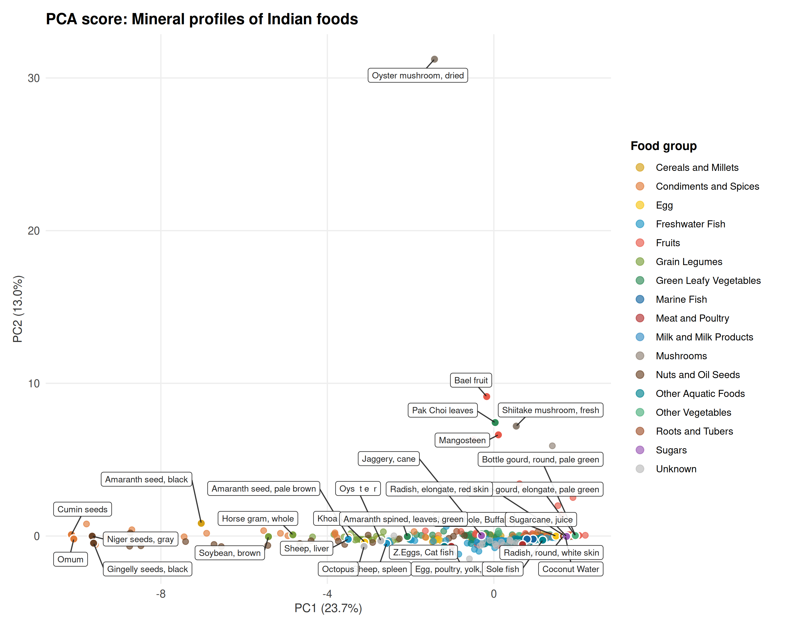
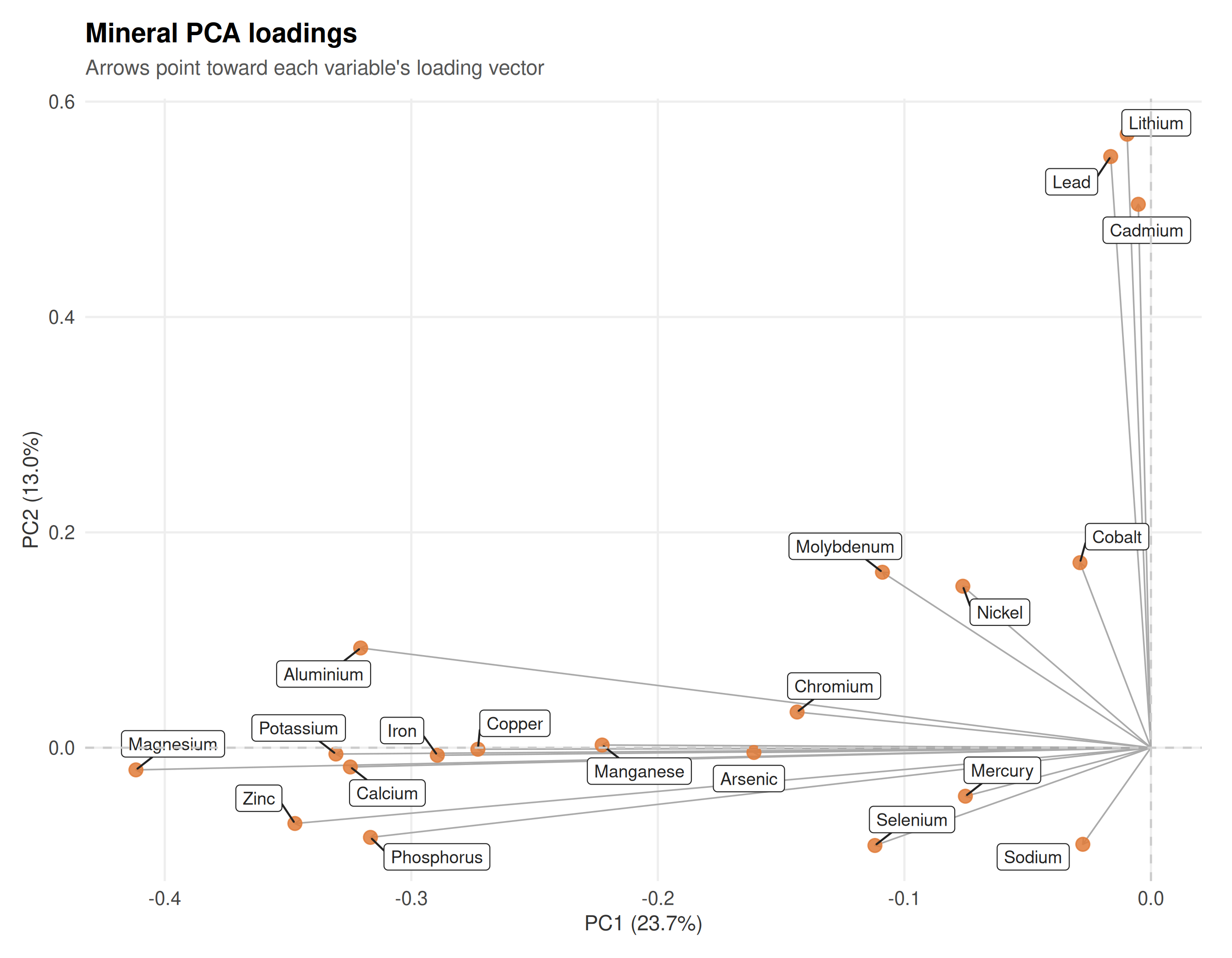
11. Mineral fingerprint PCA
All 528 IFCT foods measured for minerals, coloured by food group. PC1 and PC2 typically separate animal products (high Na, P) from plant foods (high K, Mg), with condiments pushed out by trace elements.
pca_minerals <- run_pca("minerals")
plot_pca(pca_minerals,
  title = "PCA score: Mineral profiles of Indian foods"
)
plot_pca_loadings(pca_minerals,
  label_fn = function(x) gsub("_.*", "", x),
  title = "Mineral PCA loadings"
)
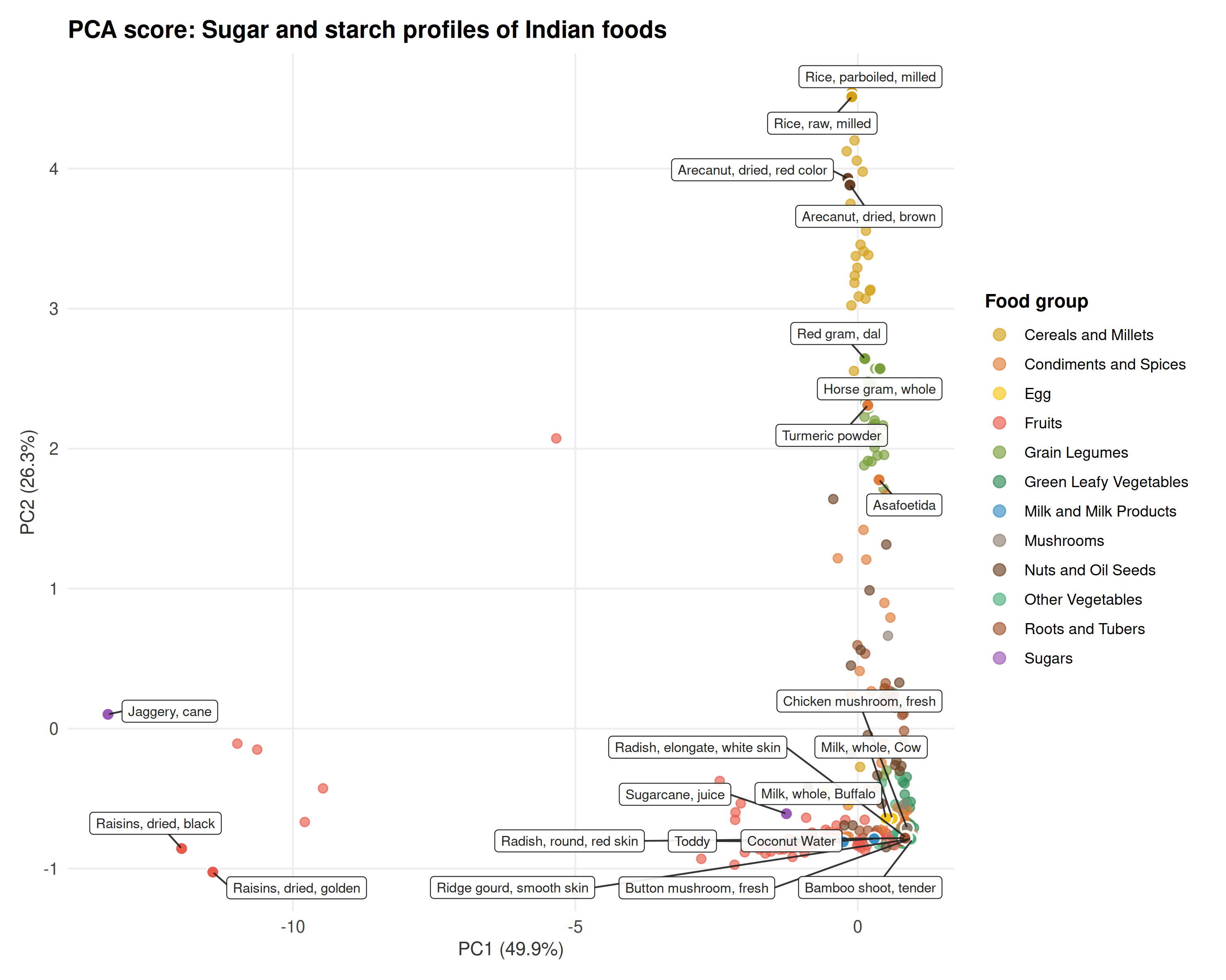
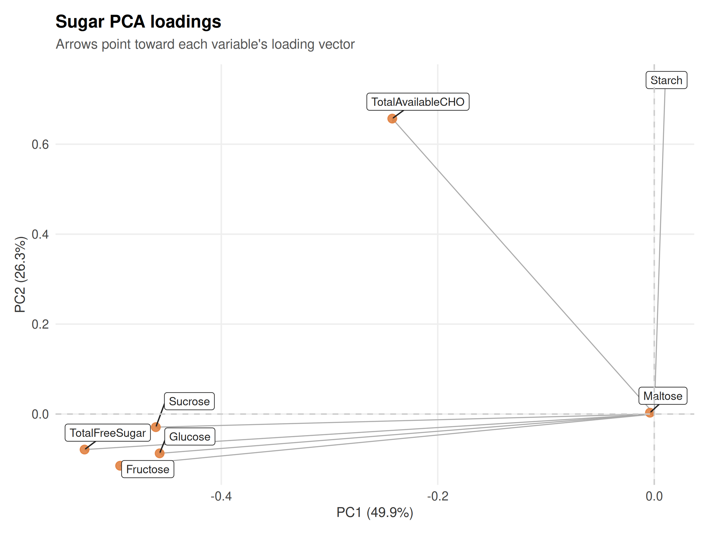
12. Sugar and starch PCA
Table 6 covers starch, total free sugars, and individual mono- and disaccharides. High-starch cereals cluster away from fruits and sugary foods, which are driven by fructose and sucrose.
pca_sugars <- run_pca("sugars", min_obs = 3L)
plot_pca(pca_sugars,
  title = "PCA score: Sugar and starch profiles of Indian foods"
)
plot_pca_loadings(pca_sugars,
  label_fn = function(x) gsub("_.*|\\(.*", "", x),
  title = "Sugar PCA loadings"
)
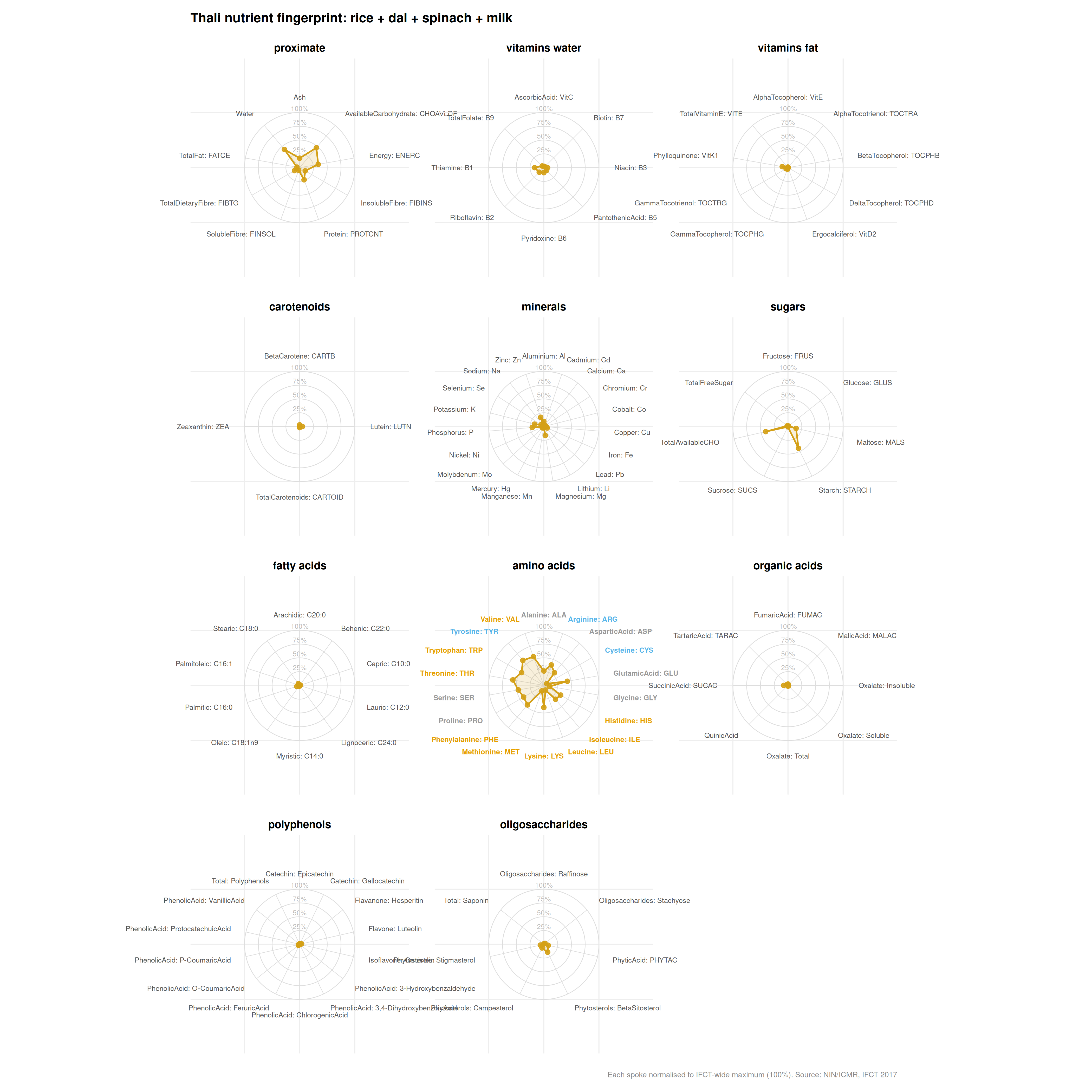
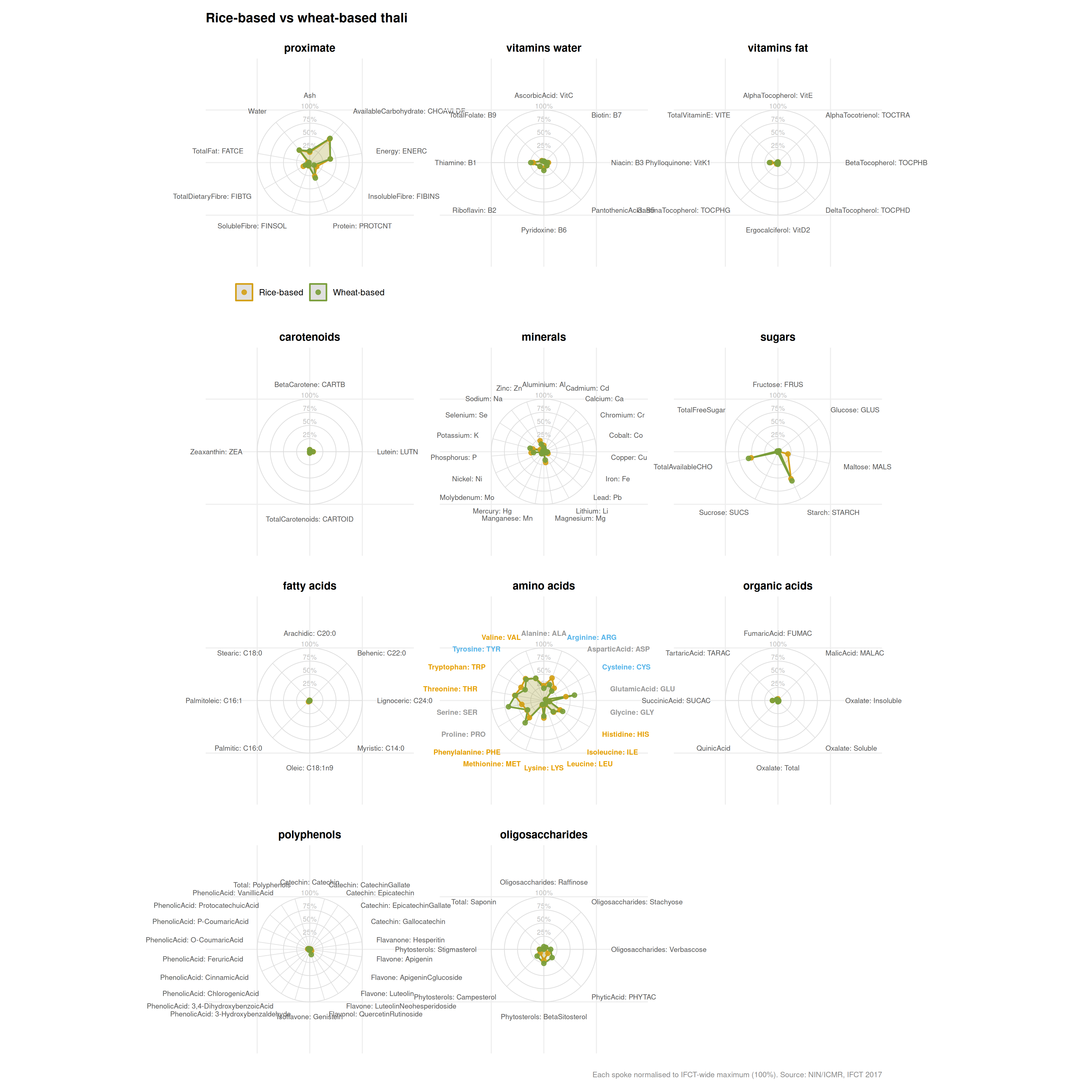
13. Thali nutrient fingerprint
Every spoke is normalised to the IFCT-wide maximum, so the shape shows where a meal sits relative to the full range of Indian foods. Pass a named list to overlay multiple meals.
thali_plot(
  c(
    "Rice"        = 150,
    "Bengal gram" = 100,
    "Spinach"     = 80,
    "Milk"        = 100
  ),
  title = "Thali nutrient fingerprint: rice + dal + spinach + milk"
)
thali_plot(
  list(
    "Rice-based"  = c("Rice" = 150, "Bengal gram" = 100, "Spinach" = 80),
    "Wheat-based" = c("Wheat flour" = 150, "Red gram" = 100, "Spinach" = 80)
  ),
  title = "Rice-based vs wheat-based thali"
)
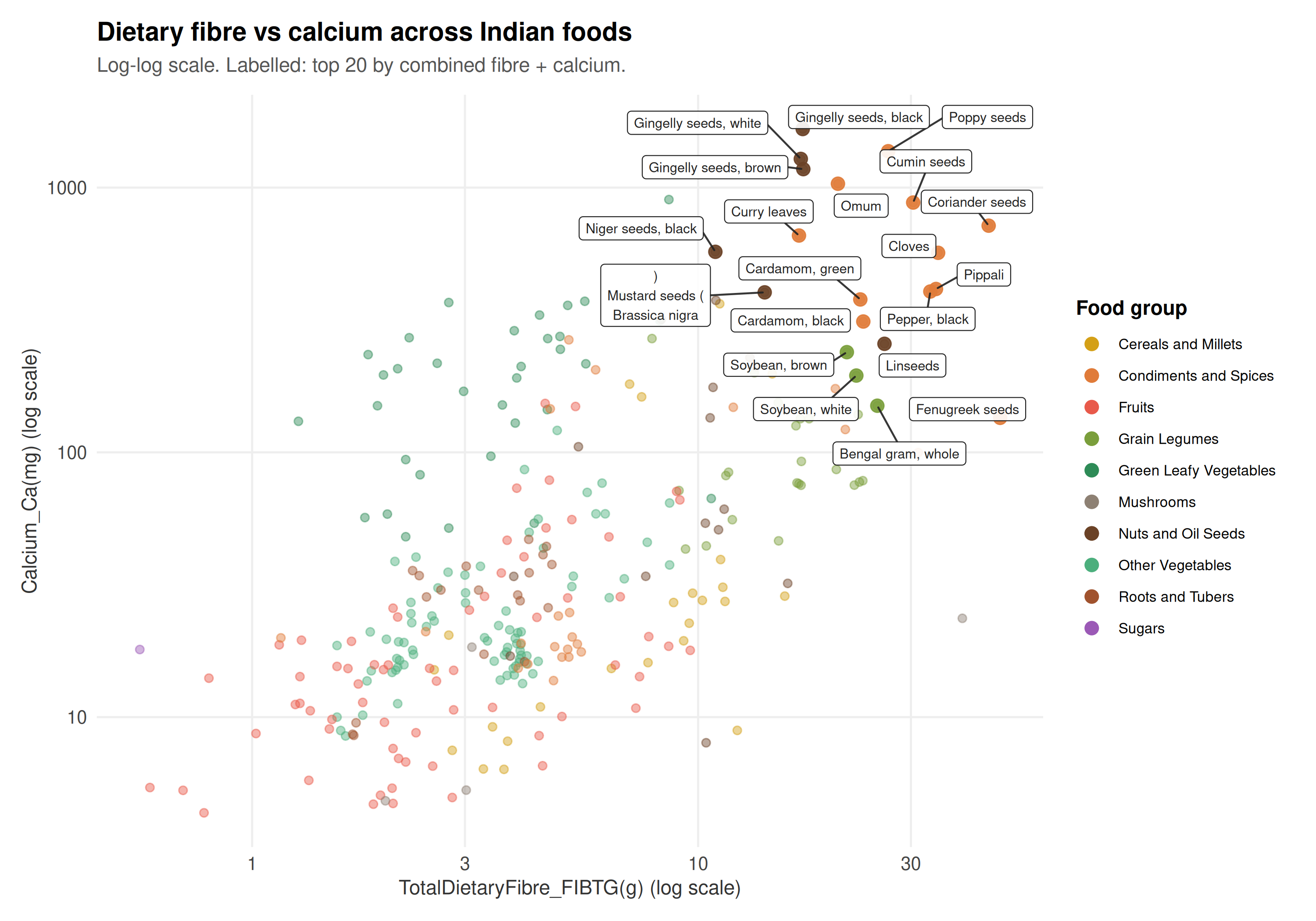
14. Cross-table join: dietary fibre vs calcium
plot_nutrient_scatter(
  x_table  = "proximate", x_col = "TotalDietaryFibre_FIBTG(g)",
  y_table  = "minerals",  y_col = "Calcium_Ca(mg)",
  log_x    = TRUE,
  log_y    = TRUE,
  title    = "Dietary fibre vs calcium across Indian foods",
  subtitle = "Log-log scale. Labelled: top 20 by combined fibre + calcium."
)
15. Food code structure
IFCT food codes encode the food group in the first letter. A001 is the first cereal, K001 the first milk product, T001 the first edible oil.
foods |>
  mutate(prefix = substr(food_code, 1, 1)) |>
  count(prefix, food_group) |>
  arrange(desc(n)) |>
  mutate(food_group = paste0("[", prefix, "] ", food_group)) |>
  select(`Food group` = food_group, `No. of foods` = n)
#> # A tibble: 19 × 2
#>    `Food group`               `No. of foods`
#>    <chr>                               <int>
#>  1 [P] Other Aquatic Foods                92
#>  2 [D] Other Vegetables                   78
#>  3 [E] Fruits                             68
#>  4 [O] Freshwater Fish                    63
#>  5 [C] Green Leafy Vegetables             34
#>  6 [G] Condiments and Spices              33
#>  7 [B] Grain Legumes                      25
#>  8 [A] Cereals and Millets                24
#>  9 [H] Nuts and Oil Seeds                 21
#> 10 [F] Roots and Tubers                   19
#> 11 [N] Marine Fish                        19
#> 12 [M] Meat and Poultry                   15
#> 13 [S] Unknown                            10
#> 14 [Q] Unknown                             8
#> 15 [R] Unknown                             7
#> 16 [J] Mushrooms                           4
#> 17 [L] Egg                                 4
#> 18 [I] Sugars                              2
#> 19 [K] Milk and Milk Products              2
Citation
If you use thali in published work, please cite both the
package and the underlying data source:
Package:
Choudhary S (2026). thali: Indian Food Composition Tables (IFCT 2017) Data for R.
R package version 0.1.0. https://github.com/saketkc/thali
Data source:
National Institute of Nutrition, ICMR (2017). Indian Food Composition Tables 2017.
NIN, Hyderabad. https://www.nin.res.in/ebooks/IFCT2017.pdf